What Happens After You Call the API
Reading order
LLM Inference Infrastructure
Previous chapter
No adjacent chapter
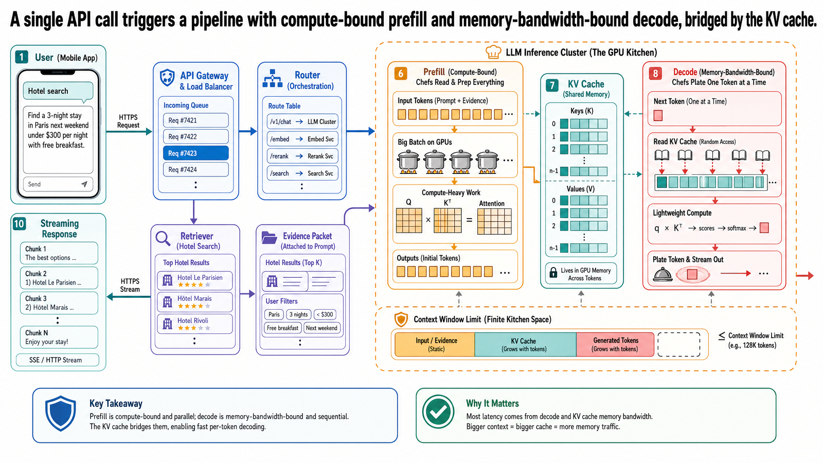
Table of Contents
- What You Already Know
- The Journey of an API Call
- How Attention Works
- The KV Cache: Why Inference Has Memory
- Two Phases of Generation: Prefill and Decode
- Prefill
- Decode
- Why LLM Inference Is Different
- The Metrics That Matter: TTFT, TPS, and ITL
- Time to first token (TTFT)
- Inter-token latency (ITL)
- Tokens per second (TPS)
- Throughput (system-level)
- Running Example: One Query Through the Pipeline
- What This Post Is Not
- Source Notes
You have built a travel copilot. A user types a query, your application sends it to an LLM provider's API, and a few seconds later a response streams back. From the application developer's perspective, that is one function call. From the infrastructure's perspective, that function call triggers a pipeline with distinct computational phases, specialized memory structures, scheduling decisions, and hardware constraints that collectively determine the latency, throughput, and cost your users experience.
This post opens that pipeline. It is not about building applications -- that is the main series. It is about understanding the machinery beneath the API so that the performance characteristics of your system stop feeling arbitrary. If you have ever wondered why the first token takes longer to appear than subsequent ones, why a long system prompt does not slow down generation as much as you expected, or why providers charge differently for input and output tokens, the answer is in this pipeline.
We will trace a single query -- a wheelchair-accessible hotel search -- from the moment it leaves your application to the moment the last token of the response arrives. Along the way, we will introduce five concepts that every subsequent post in this track depends on: attention, the KV cache, the two phases of generation, GPU resource constraints, and the metrics used to measure inference performance.
What You Already Know
This track assumes you have read Post 00-1 and Post 00-2. The main application series continues with Post 01: From Models to Compound AI Systems.
If you have read Posts 00-1 and 00-2, you already have the vocabulary this post builds on.
From Post 00-1, you know that a large language model generates text through next-token prediction. The model examines all the tokens in the sequence so far -- your input plus whatever it has already generated -- and predicts a probability distribution over the next token. It selects one, appends it, and repeats. The entire response is produced this way, one token at a time.
From Post 00-2, you know that prompts and responses share a finite context window. You know that tokens are the unit of measurement for that window and for billing. And you encountered a practical observation that many readers pass over too quickly: output tokens are more expensive than input tokens. The pricing tables in Post 00-2 showed that output costs roughly 2-10 times more than input across major providers. The stated reason was brief: "output is more expensive because each token requires sequential generation rather than parallel processing."
That sentence contains the entire motivation for this post. Input tokens can be processed in parallel. Output tokens must be generated one at a time. These two modes of processing have different computational characteristics, different hardware bottlenecks, and different memory requirements. They are, in fact, two distinct phases of inference -- and understanding them is the prerequisite for understanding every serving optimization that follows.
But to understand why these phases behave differently, we first need to understand what the model actually computes during inference. Post 00-1 described the model as a system that predicts the next token based on all preceding tokens. That is accurate, but it leaves a critical question unanswered: how does the model decide which of the preceding tokens are relevant to the current prediction?
The answer is a mechanism called attention.
The Journey of an API Call
Before we examine what happens inside the model, let us trace the full journey of a request at a high level.
Your travel copilot sends the following query to the LLM provider's API:
Show me wheelchair-accessible hotels in Kyoto under $200/night with onsen access.
This query does not arrive at the model in isolation. Your application has already assembled a complete input: a system prompt defining the copilot's behavior and formatting rules (roughly 200 tokens), a block of retrieved hotel context from your database (roughly 800 tokens), and the user's query itself (roughly 25 tokens). The total input is approximately 1,025 tokens.
Here is what happens next, in broad strokes:
The API server receives your request and passes it to a scheduler.
The scheduler places your request in a queue alongside other incoming requests. In a production deployment, dozens or hundreds of requests may be arriving concurrently. For our purposes, imagine 49 other agents submitting queries at roughly the same time.
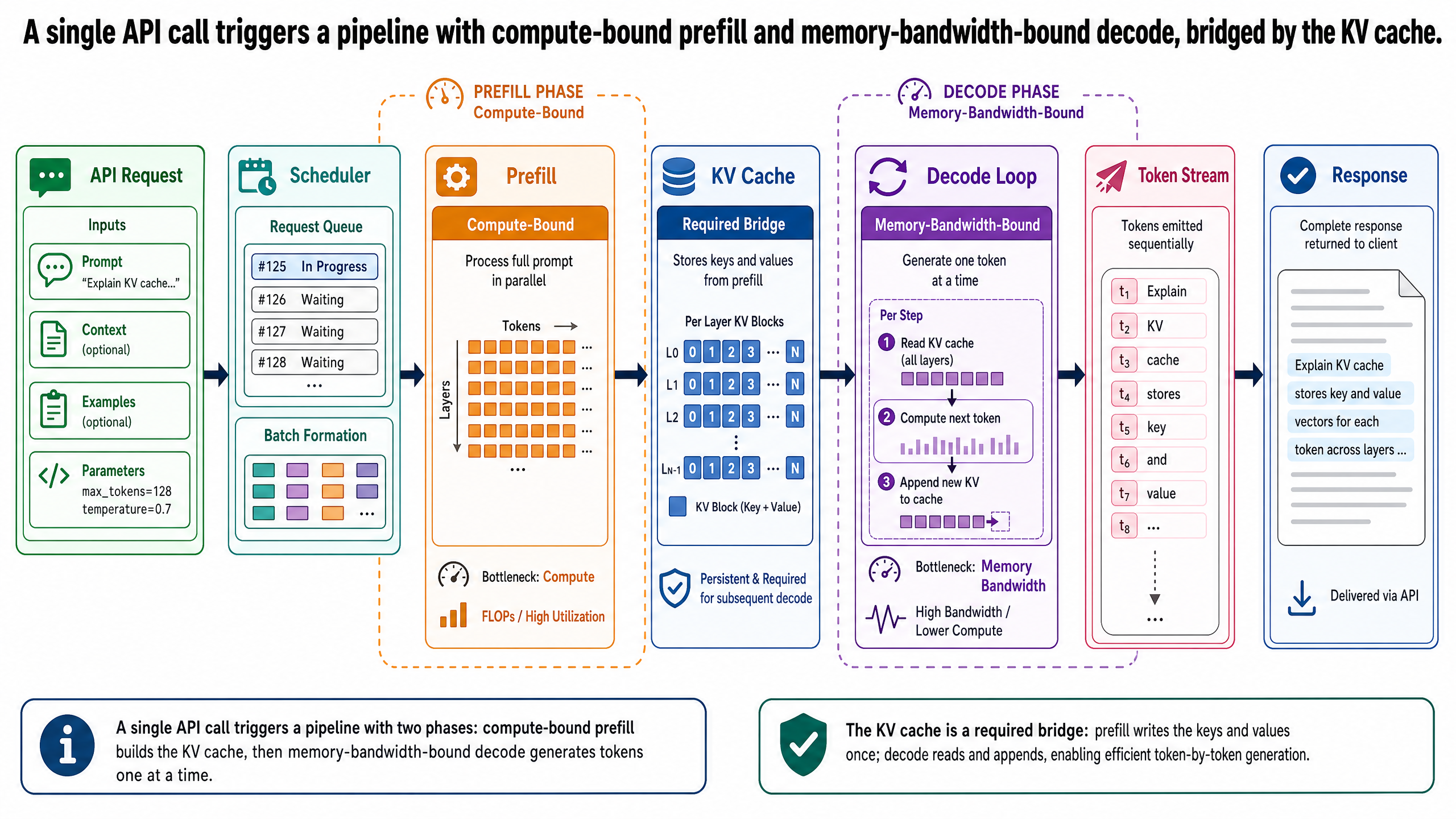
When your request reaches the front of the queue, the GPU begins processing it. The input is processed in a phase called prefill.
Prefill completes, and the model begins generating output tokens one at a time in a phase called decode. Each token streams back to your application as it is produced.
After approximately 150 output tokens, the model generates a stop token, and the response is complete.
That is the skeleton. The rest of this post fills in the details: what attention computes during each forward pass, why its outputs must be cached, how prefill and decode differ, and what the experience looks like from the user's side.
How Attention Works
During next-token prediction, the model must decide which earlier tokens in the sequence are relevant to predicting the next one. This is not a simple matter of looking at the immediately preceding word. When the model is about to generate the word "onsen" in a hotel description, the relevant context might include "wheelchair-accessible" from the user's query (to ensure the onsen facility itself is accessible), "Kyoto" from earlier in the prompt (to pull from the right geographic context), and "under $200/night" (to stay within the price filter). These tokens are scattered across the input, separated by hundreds of other tokens.
Attention is the mechanism that performs this selective focus. The name is descriptive: the model attends to the parts of the sequence that are relevant to the current prediction.
Here is how it works, conceptually. For each position in the sequence, the model computes three things:
A
queryvector: "What am I looking for?" This represents what the current position needs from the rest of the sequence.A
keyvector: "What do I contain?" This represents what a position can offer to other positions that are searching.A
valuevector: "What information do I carry?" This is the actual content that gets retrieved when a match is found.
The process is analogous to looking up relevant information in a set of notes. Imagine you are writing a hotel recommendation and you need to check whether price constraints were mentioned earlier. Your query is "price constraint." You scan your notes, and each note has a label (the key) that summarizes what it contains. When you find a note whose label matches what you are looking for -- one that says "budget: under $200/night" -- you pull the detailed information from that note (the value) and use it in your writing.
Attention works the same way, but in parallel across every position in the sequence. The model computes how well each query matches each key, and then retrieves a weighted combination of the corresponding values. Positions with highly relevant keys contribute more to the result; positions with irrelevant keys contribute almost nothing.
The foundational description of this mechanism comes from Vaswani et al.'s "Attention Is All You Need" (2017), the paper that introduced the transformer architecture. The key insight for our purposes is not the mathematics. It is that attention produces, for every token processed, a set of key and value vectors that encode that token's contribution to future predictions. Those vectors are computed during inference and must be stored somewhere -- which brings us to the most important data structure in inference infrastructure.
The KV Cache: Why Inference Has Memory
Recall that generation works one token at a time. After the model generates the first output token, it needs to generate the second. To predict the second token, it must attend to all previous tokens: the entire 1,025-token input plus the one token it just generated. To predict the third token, it attends to all 1,026 preceding tokens. And so on.
Without any optimization, each new token would require recomputing the key and value vectors for every token that came before it. The first output token requires attention over 1,025 tokens. The second requires attention over 1,026 tokens. The 150th requires attention over 1,174 tokens. The total computation grows quadratically with sequence length -- and for a 150-token response, the model would be recalculating the same key-value pairs for those original 1,025 input tokens 150 times.
This is not an edge case to optimize away. It is an impossibility to engineer around. Without caching, generation of even modest-length responses would be prohibitively slow.
The KV cache is the solution. It stores the key and value vectors that have already been computed so they can be reused for every subsequent token. When the model processes the input during prefill, it computes key and value vectors for all 1,025 input tokens and stores them in the KV cache. When it generates the first output token, it adds that token's key-value pair to the cache. When it generates the second output token, it only needs to compute the new token's query, key, and value vectors -- all the previous key-value pairs are already in the cache.
Think of it as a notebook where you keep running notes so you do not have to re-read the entire conversation from scratch every time you want to add a sentence. Each new sentence only requires consulting your notes and adding a new entry, not re-reading the full document.
The KV cache grows with every generated token. After prefill, it contains approximately 1,025 entries (one set of key-value vectors per input token, per layer of the model). After generating 150 output tokens, it contains approximately 1,175 entries. For a model with, say, 80 layers, that is 1,175 sets of key-value pairs across all 80 layers -- a substantial amount of data that must reside in GPU memory for fast access.
This is why the KV cache is not an optimization. It is a necessity. Every production inference engine -- vLLM, SGLang, TensorRT-LLM, and others -- implements KV caching as a fundamental part of its serving architecture, not as an optional acceleration.
Two Phases of Generation: Prefill and Decode
Now we can describe the two phases precisely, because the KV cache makes the distinction concrete.
Prefill
When your 1,025-token input arrives at the GPU, the model processes all 1,025 tokens in a single forward pass. This is the prefill phase, also called prompt processing. During prefill, the model computes the attention key and value vectors for every input token and stores them in the KV cache. Because all input tokens are known in advance, this computation happens in parallel -- the model processes all 1,025 tokens simultaneously rather than one at a time.
Prefill is compute-bound. The bottleneck is the GPU's arithmetic processing units. The GPU has enough data available (all 1,025 tokens sitting in memory, ready to process) but needs raw computational throughput to perform the matrix multiplications that attention and the rest of the model's layers require. Think of a kitchen during the dinner rush: the pantry is fully stocked and ingredients are ready on the counter. The constraint is how fast the chefs can chop, saute, and plate. Adding more ingredients to the counter does not help -- the chefs are already working at capacity.
Decode
After prefill completes, the model enters the decode phase, also called the generation phase. It generates output tokens one at a time. For each new token, the model runs a forward pass that computes attention using the new token's query against all the key-value pairs stored in the KV cache, generates the token, adds its key-value pair to the cache, and moves on to the next.
Each decode step processes only a single new token, but it must read the full model weights and the entire KV cache from GPU memory to do so. This is a tiny amount of computation relative to the volume of data that must be loaded.
Decode is memory-bandwidth-bound. The bottleneck is not the GPU's arithmetic units -- they finish the computation quickly -- but the speed at which data can be read from GPU memory and delivered to the processing units. Return to the kitchen analogy: now the chef is idle, waiting for a single ingredient. The pantry runner can only carry items so fast. The chef could process the ingredient in seconds, but the trip from the pantry to the counter takes longer than the cooking itself. The bottleneck has shifted from the chefs' hands to the runner's legs.
This asymmetry is the fundamental insight of LLM inference. The same hardware handles both phases, but the bottleneck is different in each. Prefill is limited by compute. Decode is limited by memory bandwidth. Optimizing one phase does not necessarily improve the other, and strategies that help prefill (more arithmetic units) may do nothing for decode (which needs faster memory access).
This also explains the cost asymmetry from Post 00-2. Output tokens are more expensive than input tokens because each output token requires its own sequential decode step, with the full memory-bandwidth overhead that entails. Input tokens, by contrast, are processed in one parallel batch during prefill. A thousand input tokens cost roughly the same compute as one prefill pass; a thousand output tokens cost a thousand sequential decode passes.
Why LLM Inference Is Different
If you have worked with other machine learning systems -- image classifiers, recommendation models, fraud detectors -- you might assume that LLM inference is just another version of "load the model, run a forward pass, return the result." It is not. LLM inference differs in five fundamental ways, and each difference creates an infrastructure problem that a later post in this track addresses.
1. Variable-length computation. An image classifier always processes a 224x224 pixel input and returns a fixed set of class probabilities. An LLM receives inputs ranging from 50 to 100,000 tokens and produces outputs ranging from 1 to 10,000 tokens. The compute and memory required for each request depend entirely on that request's specific input and output lengths. This variable-length property is the root cause of the batching problem -- you cannot simply group requests together when they will finish at different times. (Post I-01 addresses this.)
2. Two-phase resource profiles. Traditional model inference has one phase: a forward pass. LLM inference has two, with opposite hardware bottlenecks. Prefill is compute-bound; decode is memory-bandwidth-bound. A GPU configuration optimized for one phase is suboptimal for the other. This mismatch motivates the idea of running each phase on different hardware. (Post I-03 addresses this.)
3. Growing memory requirements. During decode, the KV cache grows with every generated token. A request that started with a manageable cache can, over a long generation, consume significantly more GPU memory than it initially required. The system must manage this growth dynamically -- allocating memory as it is needed, reclaiming it when requests complete, and avoiding fragmentation that wastes capacity. (Post I-02 addresses this.)
4. Cache-aware routing. In a traditional serving system, any replica can handle any request. Load balancers distribute traffic with simple strategies like round-robin. In LLM inference, if two requests share the same system prompt, a replica that has already cached the key-value vectors for that prompt can skip recomputing them. Routing a request to the wrong replica wastes the prefill computation. Intelligent routing requires awareness of what each replica has cached. (Post I-04 addresses this.)
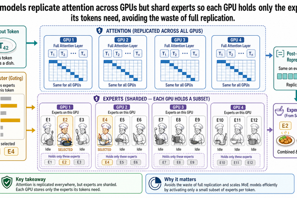
5. Architecture-dependent sharding. Some modern LLMs use a mixture-of-experts (MoE) architecture, where different parts of the model activate for different inputs. Distributing an MoE model across multiple GPUs requires different sharding strategies than distributing a dense model -- the attention layers should be replicated, while the expert layers should be partitioned. The sharding strategy is not a generic parallelism decision; it depends on the model's internal architecture. (Post I-05 addresses this.)
Each of these five differences is a reason why specialized inference engines exist. General-purpose serving frameworks that work well for image models or recommendation systems are not equipped to handle the variable lengths, two-phase computation, dynamic memory growth, cache-dependent routing, and architecture-specific sharding that LLM inference demands. Tools like vLLM, SGLang, and TensorRT-LLM were built specifically because LLM inference is a different kind of problem.
The Metrics That Matter: TTFT, TPS, and ITL
Now that you understand the two phases, you can understand the metrics that engineers use to measure inference performance. There are three that matter at the request level, plus one system-level metric.
Time to first token (TTFT)
TTFT measures the latency from the moment your application sends the request to the moment the first generated token arrives back. In our hotel search example, TTFT is the time between submitting the query and seeing the first word of the response appear.
TTFT includes everything that happens before decode begins: network transit, time spent waiting in the scheduler's queue, and the entire prefill phase. If 49 other requests are in the queue ahead of yours, the waiting time contributes to TTFT. If your input is 1,025 tokens, the prefill computation contributes to TTFT. A typical TTFT for a moderately loaded system processing our hotel query might be in the range of 100-500 ms, depending on load, input length, and hardware.
TTFT is the metric users feel most immediately. It is the silence between pressing "Send" and seeing the response start. A TTFT of 200 ms feels instant. A TTFT of 2 seconds feels sluggish. A TTFT of 10 seconds feels broken.
Inter-token latency (ITL)
ITL measures the average delay between consecutive generated tokens during the decode phase. After the first token appears, each subsequent token arrives after a small interval -- that interval is the ITL.
In our example, once the first word of the hotel response appears, ITL determines how smoothly the rest of the response streams in. An ITL of 20-40 ms produces a smooth, natural-feeling stream of text. An ITL that varies wildly -- 20 ms, then 150 ms, then 30 ms -- creates a choppy, jittery experience that users notice and dislike even when the average speed is acceptable.
ITL is primarily determined by the decode phase's memory-bandwidth bottleneck. Each decode step reads the model weights and KV cache from GPU memory, and the time that read takes sets the floor for ITL.
Tokens per second (TPS)
TPS measures how many tokens the model generates per second during decode. It is the reciprocal of ITL in simple cases: if ITL is 25 ms, TPS is roughly 40 tokens per second.
For our 150-token hotel response at 40 TPS, the decode phase takes about 3.75 seconds. Combined with a 200 ms TTFT, the user sees the first word appear almost immediately and the full response complete in under 4 seconds. That is a responsive experience.
TPS is the throughput metric at the request level. It tells you how fast a single user's response is generated.
Throughput (system-level)
At the system level, throughput measures how many total tokens (or completed requests) the system produces per second across all concurrent users. In our 50-agent scenario, throughput answers the question: how many of these agents get their responses completed per second?
Throughput is distinct from per-request TPS because it depends on how efficiently the system batches and schedules concurrent requests. A system might generate tokens at 40 TPS for a single user but, by batching 50 requests together, achieve an aggregate throughput of 1,500 tokens per second across all users. This distinction -- per-request latency versus system throughput -- is the core tension in serving optimization, and it is the subject of Post I-01.
Running Example: One Query Through the Pipeline
Now let us trace our hotel search query through the complete pipeline, labeling each metric on the timeline.
The input:
System prompt: 200 tokens (defines the copilot's role, formatting rules, accessibility guidelines)
Retrieved hotel context: 800 tokens (database results for wheelchair-accessible Kyoto hotels with onsen access)
User query: 25 tokens ("Show me wheelchair-accessible hotels in Kyoto under $200/night with onsen access.")
Total input: ~1,025 tokens
T = 0 ms. Your application sends the request to the API.
T = 5 ms. The API server receives the request and passes it to the scheduler. The scheduler sees 49 other requests currently being processed or queued. Your request enters the queue.
T = 45 ms. Your request reaches the front of the queue. The scheduler assigns it to a GPU. The prefill phase begins.
T = 45-190 ms. Prefill processes all 1,025 input tokens in parallel. The GPU performs the attention computation across every layer, producing key and value vectors for each input token at each layer. These vectors are written to the KV cache. At the end of prefill, the KV cache holds approximately 1,025 entries per layer. This is a compute-bound operation -- the GPU's arithmetic units are the bottleneck.
T = 190 ms. The first decode step runs. The model generates the first output token and streams it back to your application. TTFT = 190 ms. The user sees the beginning of the response.
T = 190-3,940 ms. The decode phase generates 149 more tokens, one at a time. Each decode step reads the model weights and the growing KV cache from GPU memory, computes attention for the new token against all cached key-value pairs, generates the token, adds its key-value pair to the cache, and streams the token to the client. Average ITL = 25 ms. The KV cache grows from ~1,025 entries to ~1,175 entries per layer.
T = 3,940 ms. The 150th token is a stop token. The response is complete. TPS = 150 tokens / 3.75 seconds = 40 tokens/second. The KV cache for this request is freed, releasing GPU memory for other requests.
The user's experience: the response started appearing in under 200 milliseconds and streamed smoothly over about 4 seconds. From the infrastructure's perspective, those 4 seconds involved two fundamentally different phases of computation, a growing memory structure, and scheduling decisions that balanced this request against 49 others.
This trace is the reference example for the rest of the track. When Post I-01 discusses how to batch this request with others, the 1,025 input tokens and 150 output tokens are the concrete numbers. When Post I-02 discusses memory management, the KV cache growing from 1,025 to 1,175 entries per layer is the concrete cost. When Post I-04 discusses prefix caching, the 200-token system prompt that is identical across all 50 agents is the concrete opportunity.
What This Post Is Not
This post introduced the inference pipeline: attention, the KV cache, prefill and decode, GPU resource characteristics, and the metrics that describe performance. It traced a single request through the full lifecycle.
It did not address what happens when the system must handle many of these requests at once.
In a production deployment, those 50 concurrent agents do not arrive in a neat, sequential queue. They arrive simultaneously, with different input lengths and unpredictable output lengths. Some requests will finish quickly; others will generate long responses. Naive batching -- grouping requests together and waiting for the longest one to finish -- wastes GPU cycles on padding, leaving most of the batch idle while the straggler completes its generation. But what happens when 50 of these queries arrive at once? The scheduler faces a batching problem that requires a fundamentally different approach.
That is the subject of Post I-01: continuous batching, the technique that schedules at the granularity of individual decode iterations rather than complete requests.
And that growing KV cache? It needs to live somewhere in GPU memory -- memory that is finite, shared across all concurrent requests, and subject to fragmentation as requests of different lengths begin and end at different times. Naive allocation wastes 60-80% of available KV cache memory.
That is the subject of Post I-02: paged KV cache management, which applies ideas from operating system virtual memory to eliminate that waste.
The inference pipeline this post described is the foundation. Everything that follows is about making it work efficiently at scale.
Source Notes
This post draws on the following primary and practitioner sources:
Vaswani, A., Shazeer, N., Parmar, N., et al. "Attention Is All You Need." NeurIPS, 2017. The foundational paper introducing the transformer architecture and the query-key-value attention mechanism. arxiv.org/abs/1706.03762
NVIDIA. "Mastering LLM Techniques: Inference Optimization." NVIDIA Developer Blog. Primary reference for the prefill/decode phase distinction and their compute-bound versus memory-bandwidth-bound resource profiles. developer.nvidia.com/blog/mastering-llm-techniques-inference-optimization
NVIDIA. "LLM Inference Benchmarking: Fundamental Concepts." NVIDIA Developer Blog. Authoritative definitions for TTFT, ITL, TPS, and throughput metrics. developer.nvidia.com/blog/llm-benchmarking-fundamental-concepts
Raschka, Sebastian. "Understanding and Coding the KV Cache in LLMs from Scratch." June 2025. Primary explanation of KV cache purpose, mechanism, and growth characteristics. magazine.sebastianraschka.com/p/coding-the-kv-cache-in-llms
BentoML. "How Does LLM Inference Work?" and "Key Metrics for LLM Inference." LLM Inference Handbook. Practitioner-oriented explanations of the two-phase inference model and metric definitions. bentoml.com/llm/llm-inference-basics/how-does-llm-inference-work and bentoml.com/llm/inference-optimization/llm-inference-metrics
Hugging Face. "Caching." Transformers documentation. Framework-level reference for KV cache implementation and behavior. huggingface.co/docs/transformers/en/cache_explanation
Yu, G., et al. "Orca: A Distributed Serving System for Transformer-Based Generative Models." OSDI, 2022. Introduced iteration-level scheduling. Referenced as historical context for continuous batching. usenix.org/conference/osdi22/presentation/yu
vLLM documentation: docs.vllm.ai. SGLang project: github.com/sgl-project/sglang. NVIDIA TensorRT-LLM: docs.nvidia.com/tensorrt-llm. Referenced as examples of specialized inference engines built for the requirements described in this post.
Huang Tzu Lin
With over five years in autonomous robotics, there's a strong passion for incorporating cutting-edge technologies and innovative approaches. Dedicated to transforming the latest research and insights into practical applications, this journey pushes the limits of possibility.
Related Posts
Stay Updated
Get the latest technical insights delivered to your inbox.