Continuous Batching: Serving Many Requests on One GPU
Reading order
LLM Inference Infrastructure
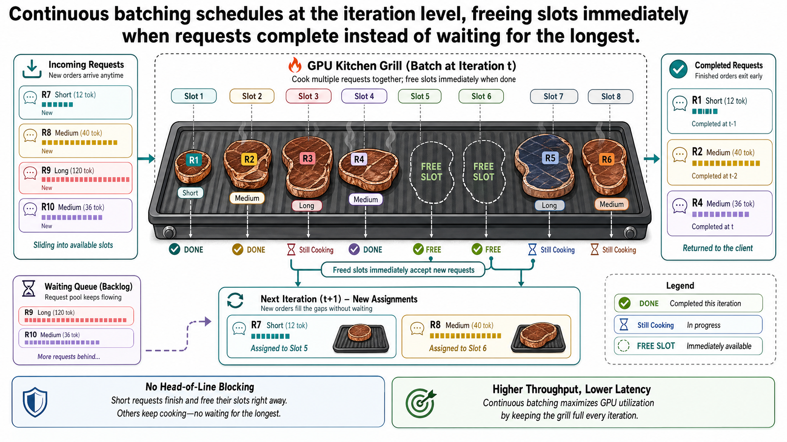
Table of Contents
- Why Batching Matters for GPU Utilization
- Naive Batching and Its Waste
- Dynamic Batching: Better Formation, Same Problem
- Continuous Batching: Iteration-Level Scheduling
- How It Works: Step by Step
- The Running Example: 8 Copilot Queries
- What the Throughput Numbers Actually Mean
- Trade-offs: Throughput Is Not Free
- What This Post Is Not
- Source Notes
Post I-00 traced a single request through the inference pipeline: prefill processed all input tokens in parallel, decode generated output tokens one at a time, and the KV cache grew with every step. At the end of that trace, we noted that 49 other agents were submitting queries at roughly the same time. That observation was not decoration. It is the central operational problem of inference serving.
When one request occupies the GPU, the hardware does useful work. But it does not do enough work. A single decode step processes one new token, yet it must load the entire model's weights from GPU memory to do so. The arithmetic units finish their computation quickly, then wait while the next round of weights is fetched. The GPU spends most of its time moving data, not computing. This is the memory-bandwidth bottleneck from I-00, and for a single request, it means the GPU's computational capacity is deeply underutilized.
The solution is batching: processing multiple requests simultaneously so that the cost of loading model weights is amortized across many requests at once. The weights are loaded once per decode step, but the computation is performed for every request in the batch. If the batch contains 8 requests, the GPU does 8 times the useful work for roughly the same memory-transfer cost.
Batching is how inference engines turn an underutilized GPU into an efficient one. But the variable-length nature of LLM generation -- the same property that makes inference fundamentally different from image classification or recommendation -- means that naive batching introduces a different kind of waste. Eliminating that waste is the subject of this post.
Why Batching Matters for GPU Utilization
Consider the alternative to batching: sequential processing. The GPU handles one request at a time. It prefills Request A, decodes all of A's output tokens, frees the KV cache, then moves to Request B. If 50 travel agents submit queries simultaneously, they wait in a queue. Request 50 does not begin until Requests 1 through 49 have each fully completed.
The problem is not just queue delay. It is hardware waste. During each decode step for a single request, the GPU loads the full model weights from memory but uses only a fraction of its arithmetic capacity. An A100 GPU can perform roughly 312 trillion floating-point operations per second, but a single decode step for one request might require only a few billion operations. The rest is idle time -- the GPU waiting for the next memory transfer.
Batching fixes this by grouping multiple requests into a single decode step. The model weights are loaded once, and the GPU computes the next token for every request in the batch simultaneously. Eight requests in a batch means eight times the useful computation per weight load. The GPU's arithmetic units, which were mostly idle during single-request decode, now have real work to do.
Think of a restaurant grill. A chef who cooks one steak at a time heats the entire grill surface but uses only a small portion of it. The heat radiating off the empty surface is pure waste. A chef who fills the grill serves more diners per hour with the same energy cost. Batching is filling the grill.
But there is a catch. Steaks on a grill are all roughly the same size and take roughly the same time. LLM requests are not.
Naive Batching and Its Waste
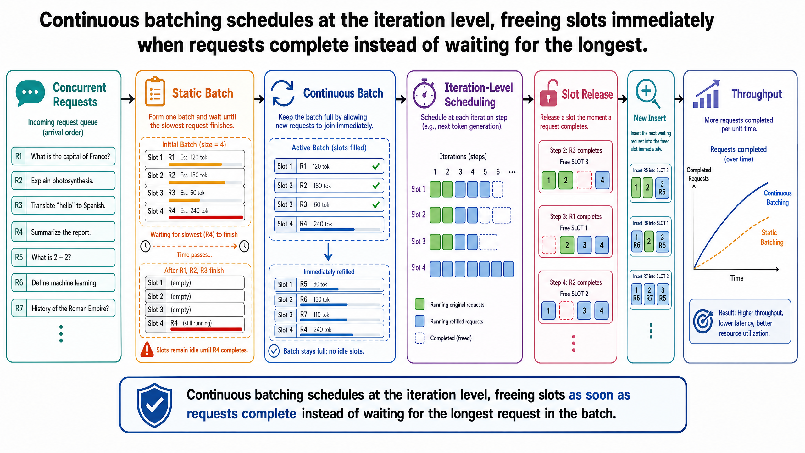
The simplest batching strategy -- sometimes called static batching -- works like this: collect a fixed number of requests, pad all input sequences to the length of the longest, and process the entire batch until every request finishes generating.
Consider 8 of the 50 travel agents submitting queries at roughly the same time:
Request — Input tokens — Output tokens
A — 800 — 20
B — 1,200 — 45
C — 950 — 80
D — 1,100 — 120
E — 750 — 150
F — 1,050 — 90
G — 900 — 60
H — 1,300 — 200
Under static batching, all 8 requests enter the batch. Prefill runs for each request, populating their KV caches. Then decode begins: at every iteration, the GPU generates one token for each of the 8 requests in lockstep.
At decode iteration 20, Request A emits its end-of-sequence token. Its response is complete -- 20 tokens, done. But the batch does not release A's slot. The batch continues, and A's slot is now filled with padding: dummy computation that produces no useful output. The GPU processes A's padding tokens at every subsequent iteration, burning cycles on work that will be discarded.
At iteration 45, Request B finishes. Another slot turns to padding. At iteration 60, Request G finishes. Then C at 80, F at 90, D at 120, E at 150. Each time a request completes, its slot becomes dead weight, but the batch grinds on.
The batch does not finish until iteration 200, when Request H -- the longest -- finally emits its stop token.
The waste is stark. Request A occupied a batch slot for 200 iterations but needed only 20. That means 180 of its 200 iterations -- 90 percent -- were padding. Across all 8 requests, the average request needed about 96 output tokens, but every request was held in the batch for 200 iterations. Roughly 52 percent of the total GPU decode computation was spent on padding tokens that contributed nothing to any response.
Meanwhile, Requests 9 through 16 -- additional agents in the queue -- waited for the entire 200-iteration batch to complete before they could begin. Their queue wait time was determined not by how long their own responses would take, but by how long Request H happened to need.
This is the fundamental inefficiency of static batching. It treats the batch as an atomic unit: nothing enters, nothing leaves, until the longest request finishes. In a workload where output lengths vary widely -- which is the norm for LLM generation -- this wastes both GPU compute (padding) and user time (queue delay).
Dynamic Batching: Better Formation, Same Problem
Dynamic batching improves how batches are assembled. Instead of waiting for a fixed number of requests, the scheduler forms batches based on time windows (batch whatever has arrived in the last 50 ms) or size triggers (batch as soon as 8 requests are queued). This reduces the time requests spend waiting to be grouped.
But dynamic batching does not change what happens after the batch is formed. Once the batch begins processing, it still runs to completion as a unit. Requests that finish early still sit in padded slots until the longest request is done. The formation is flexible; the execution is not.
Dynamic batching is a meaningful improvement over static batching for workloads with bursty arrivals, but it does not solve the core problem: variable-length outputs mean variable completion times, and batch-level scheduling wastes every cycle between a request's true completion and the batch's eventual termination.
Continuous Batching: Iteration-Level Scheduling
The insight behind continuous batching is simple: do not treat the batch as an atomic unit. Instead, re-evaluate the batch composition after every single decode iteration.
At every decode step, the scheduler asks two questions:
Did any request in the current batch just emit an end-of-sequence token?
Are there any requests waiting in the queue?
If a request completed, its slot is freed immediately. If a request is waiting, it is inserted into the freed slot. The new request begins its prefill in that slot while the remaining requests continue their decode. The batch composition changes at every iteration.
This mechanism was introduced by Yu et al. in the Orca paper (OSDI 2022) under the name iteration-level scheduling -- scheduling at the granularity of a single model forward pass rather than a complete request. The same mechanism goes by continuous batching in common usage and in-flight batching in NVIDIA's TensorRT-LLM, named for the fact that new requests begin execution while other requests are still "in flight." All three terms describe the same idea. This post uses "continuous batching" from here on.
The key shift is from batch-level scheduling to iteration-level scheduling. Static and dynamic batching schedule at the batch level: a batch starts, runs, finishes. Continuous batching schedules at the iteration level: every decode step is a scheduling decision.
How It Works: Step by Step
Return to the 8 travel-agent requests. Under continuous batching, the first 20 iterations look the same as static batching: all 8 requests are in the batch, generating tokens in lockstep.
At iteration 20, Request A completes. In static batching, A's slot would become padding. Under continuous batching, the scheduler immediately evicts A and checks the queue. Request 9 is waiting. The scheduler inserts Request 9 into A's former slot. Request 9 begins its prefill while Requests B through H continue decoding.
At iteration 45, Request B completes. The scheduler evicts B and inserts Request 10. At iteration 60, Request G completes and Request 11 enters. The pattern continues: every time a short request finishes, a waiting request immediately takes its place.
By iteration 200, when Request H finally finishes, the system has not been processing a single batch of 8 requests. It has been processing a continuously refreshed batch that has served Requests A through approximately 20 -- perhaps more, depending on the output lengths of the incoming requests. The batch stayed full throughout. No slot was ever wasted on padding.
The utilization difference is dramatic. Under static batching, GPU utilization drops as requests complete: at iteration 100, only 4 of the original 8 requests are still generating useful tokens, meaning roughly half the batch compute is padding. By iteration 180, only Request H remains active -- utilization has dropped to about 12 percent of the batch's capacity.
Under continuous batching, the batch stays full. When a slot opens, it is filled within one iteration. GPU utilization remains above 90 percent throughout because every slot is occupied by a request that is actively generating useful output.
The Running Example: 8 Copilot Queries
Apply this to the concrete throughput numbers. Suppose each decode iteration takes 25 ms (consistent with the ITL from I-00's running example).
Under static batching, the batch runs for 200 iterations: 200 x 25 ms = 5,000 ms. In those 5 seconds, the system completes 8 requests. The aggregate output is 20 + 45 + 80 + 120 + 150 + 90 + 60 + 200 = 765 tokens in 5 seconds, or about 153 tokens per second of system throughput. But the GPU was doing useful work for only about 45 percent of its decode capacity -- the rest was padding.
Under continuous batching, the same 200 iterations also take 5,000 ms. But the system does not produce only 765 tokens. As requests complete and new ones fill their slots, additional requests are being processed in parallel. If the incoming requests have similar output-length distributions, the system processes roughly 12 to 14 requests in the same 5,000 ms window, producing approximately 1,100 to 1,300 useful tokens. System throughput approximately doubles -- not because the GPU is running faster, but because it is no longer wasting cycles on padding.
For Requests 9 through 16 (the agents who would have been queued under static batching), the improvement is even more tangible. Under static batching, Request 9 waits 5 full seconds before its first token begins generating. Under continuous batching, Request 9 enters the batch at iteration 20 -- just 500 ms into the process. Its TTFT drops from over 5 seconds to well under 1 second. The queue effectively dissolves.
What the Throughput Numbers Actually Mean
You may have encountered the claim that continuous batching enables "23x throughput improvement." That number is real, but it requires decomposition.
The 23x figure comes from an Anyscale benchmark (June 2023) that compared vLLM against naive HuggingFace Transformers serving on OPT-13B with an A100 40 GB GPU. The 23x improvement reflects two optimizations working together: continuous batching (iteration-level scheduling) and PagedAttention (a memory management technique covered in I-02). The baseline -- HuggingFace Transformers without either optimization -- is the weakest reasonable comparison point.
When the same benchmark compared vLLM against TGI, which already implements continuous batching but not PagedAttention, the improvement was roughly 2x. That 2x is attributable to PagedAttention's memory efficiency, not to the batching strategy itself.
Similarly, the Orca paper (Yu et al., OSDI 2022) reported 36.9x throughput over NVIDIA FasterTransformer for GPT-3 175B. Specifically, to match a latency target of 190 ms, FasterTransformer provided 0.185 requests per second while Orca provided 6.81 requests per second. This is a comparison of iteration-level scheduling against request-level scheduling in a distributed serving context for a 175-billion-parameter model.
Both numbers are legitimate measurements. Neither is a universal statement about what continuous batching alone delivers. The lesson is to always ask: "compared to what baseline, on what model, on what hardware?" A 23x improvement over a naive baseline and a 2x improvement over a system that already has continuous batching are both true -- and they tell very different stories.
Every major inference engine now implements continuous batching: vLLM, TensorRT-LLM, SGLang, TGI. The technique is table stakes, not a differentiator. The frontier has moved to the problems that continuous batching exposes -- memory management, phase interference, and cache-aware routing -- which are the subjects of the next three posts.
Trade-offs: Throughput Is Not Free
Continuous batching optimizes for aggregate system throughput, not individual request latency. There are trade-offs to understand.
Batch size and per-request latency. Each decode iteration processes the entire batch. A larger batch means more computation per iteration, which means each iteration takes slightly longer. If a single-request decode step takes 20 ms, a batch of 32 requests might take 30 ms per step. The individual request generates tokens more slowly (higher ITL), but the system produces 32 tokens per step instead of 1. Throughput scales; per-request latency degrades modestly.
Queue pressure under heavy load. When requests arrive faster than the GPU can process them, the batch stays full and the queue grows. A newly arrived request must wait for a slot to open -- which happens only when a currently running request completes. Under sustained heavy load, queue wait time can dominate TTFT. The system must implement backpressure -- throttling or rejecting requests -- to maintain latency targets. TensorRT-LLM addresses this with scheduler policies like GUARANTEEDNOEVICT, which prevents the scheduler from evicting partially completed requests to make room for new ones.
Batch saturation. There is a ceiling. Adding more requests to the batch improves throughput only until GPU memory is exhausted. Every concurrent request in the batch has a KV cache that must reside in GPU memory. At some point, the memory is full and no additional requests can be admitted regardless of available compute. This memory ceiling is the direct motivation for I-02: efficient KV cache management that packs more concurrent requests into the same memory budget.
Prefill-decode interference. When a new request enters the batch under continuous batching, it must run its prefill phase. Prefill is compute-bound; decode is memory-bandwidth-bound. Running both simultaneously on the same GPU can cause interference: the prefill computation contends with decode for GPU resources, potentially causing latency spikes for the requests that are mid-generation. This interference is the direct motivation for I-03: separating prefill and decode onto different hardware.
What This Post Is Not
This post taught the scheduling mechanism that keeps the GPU full: continuous batching replaces batch-level scheduling with iteration-level scheduling, eliminating padding waste and dramatically improving system throughput.
It did not teach how the KV cache for all those concurrent requests is stored efficiently. Continuous batching keeps the batch full, which means more requests are in flight simultaneously, which means more KV caches competing for GPU memory. Naive memory allocation wastes 60 to 80 percent of available KV cache space through fragmentation. Where does all that memory go, and how do inference engines fit more into the same budget? That is the subject of Post I-02: paged KV cache management, which applies ideas from operating system virtual memory to solve exactly this problem.
And when prefill and decode share the same GPU -- as they do in the continuous batching scheme described here -- they can interfere with each other. A large prefill for a newly arrived request can stall token generation for every other request in the batch. Separating the two phases onto different hardware is the subject of Post I-03.
Continuous batching is the foundation. Every optimization that follows in this track builds on the assumption that the inference engine is already scheduling at the iteration level. The next three posts address the problems that this foundation exposes.
Source Notes
This post draws on the following primary and practitioner sources:
Yu, G., Jeong, J. S., Kim, G., Kim, S., and Chun, B. "Orca: A Distributed Serving System for Transformer-Based Generative Models." OSDI, 2022. The paper that introduced iteration-level scheduling. The 36.9x throughput figure over FasterTransformer (GPT-3 175B, 190 ms latency target) is from this paper. usenix.org/conference/osdi22/presentation/yu
Anyscale. "How Continuous Batching Enables 23x Throughput in LLM Inference While Reducing p50 Latency." June 2023. The benchmark that popularized the term "continuous batching." The 23x figure compares vLLM (continuous batching + PagedAttention) against naive HuggingFace Transformers on OPT-13B / A100 40 GB. anyscale.com/blog/continuous-batching-llm-inference
Anyscale. LLM Continuous Batching Benchmarks (reproduction code). github.com/anyscale/llm-continuous-batching-benchmarks
NVIDIA. "Mastering LLM Techniques: Inference Optimization." NVIDIA Developer Blog. Reference for GPU utilization characteristics and the batching-utilization relationship. developer.nvidia.com/blog/mastering-llm-techniques-inference-optimization
NVIDIA TensorRT-LLM documentation. Reference for "in-flight batching" terminology and scheduler policies (MAXUTILIZATION, GUARANTEEDNO_EVICT). nvidia.github.io/TensorRT-LLM/overview.html
BentoML. "Static, Dynamic and Continuous Batching." LLM Inference Handbook. Practitioner-oriented definitions for the three batching strategies. bentoml.com/llm/inference-optimization/static-dynamic-continuous-batching
vLLM documentation. docs.vllm.ai. SGLang project. sgl-project.github.io. Referenced as implementations of continuous batching showing the technique's universality across inference engines.
LMSYS. "SGLang v0.4: Zero-Overhead Batch Scheduler." December 2024. Reference for the state of the art in continuous batching scheduler design. lmsys.org/blog/2024-12-04-sglang-v0-4
Huang Tzu Lin
With over five years in autonomous robotics, there's a strong passion for incorporating cutting-edge technologies and innovative approaches. Dedicated to transforming the latest research and insights into practical applications, this journey pushes the limits of possibility.
Related Posts
Stay Updated
Get the latest technical insights delivered to your inbox.