Prefill-Decode Disaggregation: Splitting the Two Stages of Inference
Reading order
LLM Inference Infrastructure
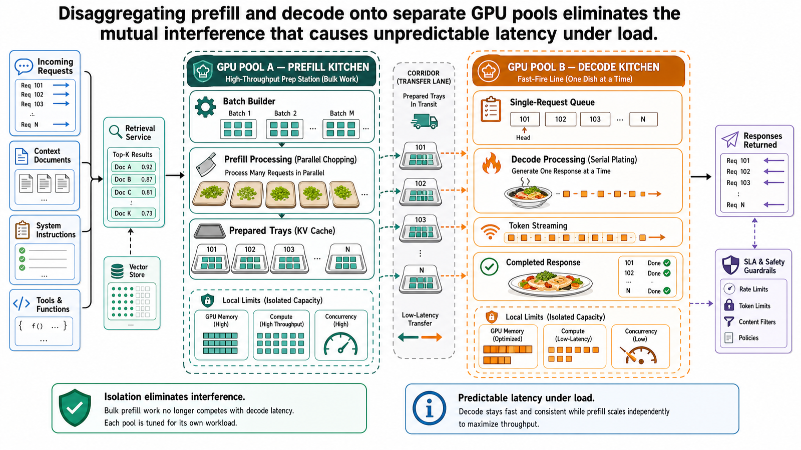
Table of Contents
- Two Phases With Different Properties
- The Interference Problem
- What Happens When You Mix Them
- Disaggregation: Separate Pools
- KV Cache Transfer: The Cost
- Goodput: The Metric That Matters
- Running Example: 50 Copilot Queries, Mixed Versus Disaggregated
- Mixed pool
- Disaggregated pools
- When To Disaggregate (and When Not To)
- What This Post Is Not
- Source Notes
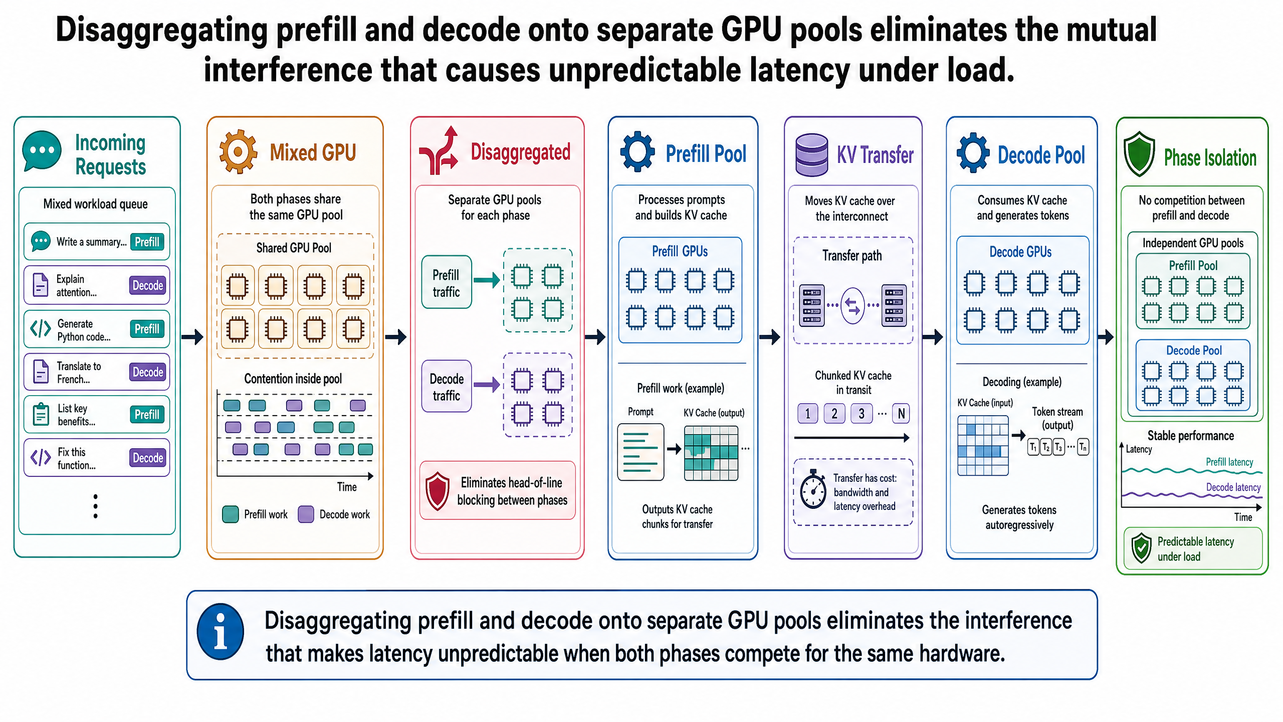
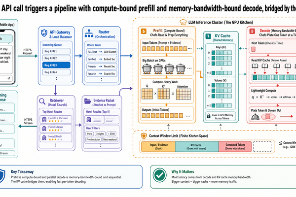
Post I-00 established that LLM inference has two phases with fundamentally different resource profiles. Prefill processes all input tokens in parallel and is compute-bound -- the GPU's arithmetic units are the bottleneck. Decode generates tokens one at a time and is memory-bandwidth-bound -- the bottleneck is reading model weights and the KV cache from GPU memory. Post I-01 introduced continuous batching, which keeps the GPU full by scheduling at the iteration level rather than the batch level. Post I-02 showed how PagedAttention eliminates memory waste so more requests can be active simultaneously.
Together, these optimizations transformed GPU utilization. But they also created a new problem. Continuous batching keeps the batch full, which means prefill operations for newly arriving requests run alongside decode operations for active requests -- on the same GPU, competing for the same resources. The two phases have opposite bottlenecks, and forcing them to share hardware means neither runs at its best. This interference is the subject of this post.
Two Phases With Different Properties
A brief recap, because the rest of the post depends on it.
When a request arrives, the model processes all input tokens in a single forward pass during prefill. This is the compute-bound phase. The GPU has plenty of data available -- all the input tokens are ready -- but its arithmetic units must churn through the matrix multiplications that attention and the model's layers require. From I-00's kitchen analogy: the pantry is fully stocked, the constraint is how fast the chefs can chop and plate.
After prefill populates the KV cache, the model enters decode. Each step generates one token, but it must read the full model weights and the growing KV cache from GPU memory to do so. The arithmetic units finish quickly; the bottleneck is the speed at which data can be loaded from memory. The chef is idle, waiting for the runner to bring a single ingredient from the pantry.
These are not two workloads that happen to be different. They are workloads with opposite resource profiles. Prefill wants compute throughput. Decode wants memory bandwidth. A GPU configuration optimized for one is suboptimal for the other. And yet, in a standard inference engine using continuous batching, both phases run on the same hardware at the same time.
The Interference Problem
Continuous batching made GPU utilization dramatically better. It also made prefill-decode co-scheduling more frequent. Every time a new request enters the batch, its prefill runs alongside the ongoing decodes of every other active request. For short prompts at low concurrency, this interference is barely noticeable. For long prompts at high concurrency, it is the dominant source of latency variance.
The interference is mutual. When a compute-heavy prefill runs, it saturates the GPU's arithmetic units, delaying the memory-bandwidth-bound decode iterations for all co-scheduled requests. Those decode requests experience ITL spikes -- their streaming responses stutter. Simultaneously, the decode operations' memory-bandwidth demands slow down the prefill. Both phases degrade each other.
This creates a coupling between TTFT and ITL that makes the system fundamentally difficult to tune. Prioritize prefill to keep TTFT low, and active decodes stall. Throttle prefill to protect decode, and new requests wait longer for their first token. The scheduler cannot optimize for both metrics at once because the underlying problem is physical: two workload types with opposite resource needs are contending for the same hardware.
DistServe (Zhong et al., OSDI 2024), the paper that formalized disaggregation as an architecture, describes this as "strong prefill-decoding interferences" that "couple the resource allocation and parallelism plans for both phases." Splitwise (Patel et al., ISCA 2024), which arrived at the same insight independently from a hardware-efficiency perspective, characterizes the problem differently but reaches the same conclusion: "each phase of generative LLM inference has distinct latency, throughput, memory, and power characteristics," and co-locating them forces both into a compromise that serves neither well.
What Happens When You Mix Them
Return to the 50 concurrent travel agents from the running example. During peak booking season, queries arrive continuously. Most are routine: 600 to 1,000 input tokens, generating 100 to 200 output tokens. The system handles them well under continuous batching. ITL holds steady at around 25 ms. Responses stream smoothly.
Then a senior travel agent submits a complex multi-leg itinerary query. The copilot's system prompt (200 tokens), retrieved hotel database context (1,200 tokens), rail pass schedules (400 tokens), and the detailed user query (200 tokens) total approximately 2,000 input tokens -- roughly twice the average.
On a mixed GPU running continuous batching, here is what happens:
The 2,000-token query enters the batch alongside 7 active decode requests from other agents.
Prefill begins. The GPU's compute units are saturated processing 2,000 tokens through all attention layers. This prefill takes approximately 80 ms of compute-intensive processing.
During those 80 ms, the 7 decode requests cannot get their memory-bandwidth-bound iterations serviced efficiently. Their ITL jumps from a steady 25 ms to 90 ms or more. The streaming responses those agents are reading visibly stutter. Two agents experience gaps of 200 ms or more in their output -- long enough to notice and wonder if the system is broken.
After the long prefill completes, the new request begins decoding and ITL settles back to 25 ms for everyone. The system feels normal again.
But the damage compounds. Under sustained load, long prefills arrive every few seconds. Each one causes the same interference pattern. TTFT and ITL become unpredictable. The system hits its aggregate throughput target -- it is processing requests -- but it violates latency SLOs on 30 to 40 percent of them.
This is head-of-line blocking: a long prefill for one request delays decode iterations for all other active requests on the same GPU. The term is borrowed from networking, where a large packet at the front of a queue delays every packet behind it. The analogy is precise. The long prefill is the large packet. The co-scheduled decodes are the packets stuck waiting.
The problem is not that the system is slow in aggregate. The problem is that it is unpredictable. Seven users experience degraded service every time one user submits a long prompt. The throughput numbers look fine in a monitoring dashboard; the user experience does not.
Disaggregation: Separate Pools
The solution is physical separation. Assign prefill and decode to different GPU pools. Each pool is configured for the resource profile of its phase.
The prefill pool handles input processing. Its GPUs are configured for compute throughput -- high parallelism, optimized for the large matrix operations that attention over thousands of input tokens demands. The prefill pool does not need to maintain long-lived KV caches for many concurrent decode streams. Its job is to process input, compute the KV cache, and hand it off.
The decode pool handles token generation. Its GPUs are configured for memory-bandwidth efficiency -- optimized for the repeated pattern of loading model weights and KV cache, computing one token, and doing it again. The decode pool does not need to handle compute-intensive prefill bursts. Its workload is steady and predictable.
The architecture works like this: when a request arrives, the scheduler routes it to the prefill pool. A prefill GPU processes all input tokens and computes the KV cache. Once prefill completes, the KV cache is serialized and transferred over the network to a decode GPU. Decode begins on the decode GPU, and the response streams back to the user.
The result is phase isolation: each phase runs without affecting the other's performance. The 2,000-token itinerary query's prefill runs on a prefill GPU. The 7 agents who are mid-decode on the decode pool are undisturbed. Their ITL stays at 25 ms throughout. No stuttering. No interference. No unpredictable latency spikes.
Independent scaling is the second structural advantage. In a co-located system, adding a GPU adds capacity for both prefill and decode equally -- whether the workload needs it or not. With disaggregated pools, the ratio can match the workload. A prompt-heavy workload (long inputs, short outputs) needs more prefill GPUs. A generation-heavy workload (short inputs, long outputs) needs more decode GPUs. Splitwise further proposes using different hardware tiers: latest-generation GPUs for the compute-bound prefill pool, and less expensive hardware for the memory-bandwidth-bound decode pool, potentially reducing cost while maintaining or improving throughput.
This is no longer just a research concept. By 2025-2026, disaggregated serving had moved into production-oriented inference stacks. NVIDIA Dynamo documents disaggregated serving as a first-class design, and vLLM exposes disaggregated prefill with multiple KV-transfer backends. That does not mean every deployment should use it, or that every framework implements it the same way. It means the pattern has matured from paper architecture into a practical option that production teams can evaluate against their workload, interconnect, and latency SLOs.
KV Cache Transfer: The Cost
Disaggregation is not free. It introduces a step that co-located systems do not have: after prefill completes, the KV cache must be serialized and sent from the prefill GPU to the decode GPU over a network connection.
This transfer has a concrete size. Recall from I-02 that the KV cache stores key and value vectors for every input token across every layer of the model. The memory per token follows a formula: 2 (keys and values) multiplied by the number of layers, the number of KV heads, the head dimension, and the precision in bytes. For a 70-billion-parameter model like Llama 2 70B processing 2,000 input tokens in FP16 precision, the KV cache is approximately 1.25 GB. That is for a single request.
Whether this transfer is fast enough depends entirely on the interconnect. Within a single node using high-speed NVLink, the transfer is nearly invisible. DistServe reports that KV cache transfer overhead is less than 0.1 percent of total serving time when prefill and decode GPUs are within the same node using intra-node NCCL bandwidth. At that overhead, the transfer is a rounding error.
But not all deployments are single-node. On slower inter-node links, the math changes. Splitwise calculates that a single 512-token request on OPT-66B produces approximately 1.13 GB of KV cache. At 10 requests per second, sustaining that transfer rate demands roughly 90 Gbps of bandwidth to avoid bottlenecking. If the available bandwidth is lower, KV cache transfer becomes a chokepoint that adds latency instead of removing it.
The research community has developed mitigation strategies. Splitwise overlaps KV cache transfer with prefill computation by triggering asynchronous layer-wise transfers: as soon as one layer's KV vectors are computed during prefill, they begin transferring to the decode GPU while the next layer's computation proceeds. This hides much of the transfer latency behind computation that is already happening. vLLM supports multiple transfer backends -- NCCL, NixL, and Mooncake -- each optimized for different network topologies.
The honest summary: within a well-connected node, KV cache transfer is cheap enough to ignore. Across nodes with limited bandwidth, or at very high request rates, it is a real constraint that must be measured, not assumed away.
Goodput: The Metric That Matters
This is a good moment to introduce a metric that captures what disaggregation actually optimizes.
Raw throughput -- requests processed per second -- does not tell you whether users are having a good experience. A system that processes 100 requests per second but violates TTFT targets on 40 percent of them is not serving well. The monitoring dashboard shows healthy throughput. The users see stuttering, delays, and unpredictable response times.
DistServe introduced goodput to address this gap. Goodput is the maximum request rate at which a target percentage of requests -- for example, 90 percent -- meet both TTFT and TPOT (time per output token, equivalent to ITL) SLOs simultaneously. It captures the intersection of throughput and latency quality. Only requests that meet latency targets count.
Goodput is the metric that makes disaggregation's value legible. A co-located system and a disaggregated system might have similar raw throughput. But if the co-located system violates latency SLOs on a third of its requests due to prefill-decode interference, its goodput is dramatically lower. Disaggregation improves goodput by eliminating the interference that causes those violations -- even when the raw request rate is unchanged.
The research results are significant when read through this lens. DistServe achieves up to 7.4 times more goodput, or can serve the same request rate with 12.6 times tighter SLO bounds, compared to state-of-the-art co-located systems, across various LLMs and latency requirements. The "or" matters: these are two ways of measuring the improvement, not both achieved simultaneously. Splitwise, approaching the problem from hardware efficiency, reports up to 1.4 times higher throughput at 20 percent lower cost, or 2.35 times more throughput under the same power and cost budgets. Both sets of numbers are real. Both require understanding the baselines and conditions they were measured against.
Running Example: 50 Copilot Queries, Mixed Versus Disaggregated
Return to the concrete scenario. The same 2,000-token itinerary query, the same 50 concurrent agents, the same hardware. The only difference is the serving architecture.
Mixed pool
The 2,000-token query enters the batch alongside 7 active decode requests. Prefill runs for approximately 80 ms, during which the 7 decode requests experience ITL spikes from 25 ms to 90 ms or more. Short queries queued behind the long prefill also experience elevated TTFT. Under sustained load with occasional long prompts:
P90 TTFT: 320 ms
P90 ITL: 85 ms
Goodput at target SLOs (TTFT < 200 ms, TPOT < 50 ms): 12 requests per second
The system processes requests. It just violates latency targets on a large fraction of them.
Disaggregated pools
The 2,000-token query routes to the prefill pool. A prefill GPU processes all 2,000 tokens in approximately 80 ms -- the same compute cost. The resulting KV cache (approximately 1.25 GB for the 70B-class model) transfers to the decode pool over intra-node NVLink in roughly 5 ms. Decode begins on a decode-optimized GPU.
Meanwhile, the 7 agents on the decode pool are undisturbed throughout. Their ITL remains at a steady 25 ms. No stuttering, no spikes, no interference.
P90 TTFT: 130 ms
P90 ITL: 28 ms
Goodput at the same SLOs: 45 requests per second
The goodput improvement is 3.75 times -- not because the hardware is faster, but because the system no longer wastes latency budget on interference. The senior agent's TTFT is approximately 85 ms (80 ms prefill plus 5 ms transfer), and the 7 other agents never notice the long prefill happened at all.
When To Disaggregate (and When Not To)
Disaggregation is not universally better. It adds infrastructure complexity -- two pools, a transfer mechanism, a routing layer, and a coordination protocol. It increases total GPU memory consumption because both pools must hold the full model weights. And it introduces a network hop between prefill and decode that does not exist in a co-located system. These costs are justified only when the workload creates enough interference to make them worth paying.
Disaggregation helps when:
The workload has high concurrency with mixed prompt lengths, so long prefills frequently interfere with active decodes. The application has strict latency SLOs where P90 or P99 targets matter -- customer-facing streaming applications, copilots, real-time assistants. The cluster has sufficient inter-GPU bandwidth (high-speed NVLink or equivalent) to make KV cache transfer cheap. The prompt-to-output ratio varies enough that independent pool scaling provides meaningful cost savings.
Disaggregation does not help when:
Concurrency is low and interference is rare. If the system handles 5 to 10 concurrent requests, the probability of a long prefill colliding with active decodes is low, and the interference, when it occurs, is brief. Short prompts dominate the workload. If prefill takes 5 ms per request, the interference window is too small to cause meaningful ITL spikes. A co-located system with continuous batching handles this workload cleanly. Inter-GPU bandwidth is limited. If the KV cache transfer becomes a bottleneck, disaggregation adds latency instead of removing it. The application does not have differentiated latency requirements. Batch processing workloads -- offline summarization, bulk extraction, dataset generation -- care about aggregate throughput, not P90 TTFT. Disaggregation's goodput advantage is irrelevant when nobody is watching the stream.
BentoML's LLM Inference Handbook warns explicitly: if the workload is too small or the GPU setup is not tuned for disaggregation, performance can drop by 20 to 30 percent. The overhead of KV cache transfer and the infrastructure complexity of maintaining two pools can outweigh the benefits when interference is not a significant problem.
A brief counter-example makes this concrete. Consider 10 agents submitting short queries -- 300 tokens each -- at low concurrency. Prefill takes approximately 5 ms per query, far too short to cause meaningful interference with co-scheduled decodes. Disaggregation would add roughly 2 ms of transfer overhead per request for minimal benefit. A co-located system with continuous batching is simpler, cheaper, and equally effective.
The right framing is not "disaggregation is better" but "disaggregation trades infrastructure complexity for latency predictability." Whether that trade is worth making depends on the workload, the hardware, and the SLOs. The original DistServe research captures this precisely: disaggregation can lead to much better performance or much more predictable performance. The "or" is important -- it is not always both simultaneously.
What This Post Is Not
This post taught why prefill-decode interference occurs, how disaggregation eliminates it by physically separating the two phases, what the KV cache transfer costs, and when the trade-off is favorable. It introduced goodput as the metric that captures what disaggregation optimizes -- serving quality under latency constraints, not just raw request throughput.
It did not cover how to implement disaggregation in a specific engine. vLLM, SGLang, NVIDIA Dynamo, and Ray Serve each have their own configuration, their own transfer backends, and their own routing strategies. Those are implementation details, not architectural concepts.
It did not cover prefix-aware routing. With disaggregated pools, there is another opportunity: what if the scheduler routes requests to decode GPUs that already have their prefix cached? If two consecutive requests share the same system prompt, and the second request lands on a different decode GPU, the KV cache for that shared prefix must be re-prefilled or re-transferred from scratch. Routing requests to cache-hot replicas eliminates that waste. That is the subject of Post I-04.
And it did not cover how disaggregation interacts with mixture-of-experts architectures, where the model itself is partially activated and sharding strategies add another dimension to pool design. That is the subject of Post I-05.
Disaggregation decides which pool handles each phase. The next question is which specific GPU within a pool receives the request -- and that decision depends on what is already cached there. That is where we go next.
Source Notes
This post draws on the following primary and practitioner sources:
Zhong, Y., Liu, S., Chen, J., Hu, J., Zhu, Y., Liu, X., Jin, X., and Zhang, H. "DistServe: Disaggregating Prefill and Decoding for Goodput-optimized Large Language Model Serving." OSDI, 2024. Primary source for the disaggregation architecture, the goodput metric, interference characterization, the 7.4x goodput / 12.6x tighter SLO results (compared to state-of-the-art co-located systems), and the KV cache transfer overhead measurement (<0.1% with intra-node NCCL). arxiv.org/abs/2401.09670
Patel, P., Choukse, E., Zhang, C., Shah, A., Goiri, I., Maleki, S., and Bianchini, R. "Splitwise: Efficient Generative LLM Inference Using Phase Splitting." ISCA, 2024. Primary source for hardware-perspective phase characterization, layer-wise KV cache transfer (asynchronous overlap with prefill computation), heterogeneous hardware for disaggregated pools, the 1.4x throughput / 20% lower cost result, and concrete KV cache sizing (1.13 GB for a 512-token OPT-66B request requiring 90 Gbps at 10 req/s). arxiv.org/abs/2311.18677
NVIDIA. "Mastering LLM Techniques: Inference Optimization." NVIDIA Developer Blog. Reference for the compute-bound versus memory-bandwidth-bound characterization of prefill and decode phases. developer.nvidia.com/blog/mastering-llm-techniques-inference-optimization
NVIDIA. "Introducing NVIDIA Dynamo: A Low-Latency Distributed Inference Framework for Scaling Reasoning AI Models." NVIDIA Developer Blog. Reference for Dynamo's production disaggregation support, announced at GTC 2025. developer.nvidia.com/blog/introducing-nvidia-dynamo-a-low-latency-distributed-inference-framework-for-scaling-reasoning-ai-models
vLLM. "Disaggregated Prefilling." vLLM Documentation. Reference for vLLM's production disaggregation implementation, transfer backends (NixlConnector, P2pNcclConnector, MooncakeConnector), and the observation that disaggregated prefilling is "a much more reliable way to control tail ITL compared to chunked prefill." docs.vllm.ai/en/latest/features/disagg_prefill
BentoML. "Prefill-decode disaggregation." LLM Inference Handbook. Practitioner-validated warning that performance can drop 20-30% when disaggregation is applied to inappropriate workloads (low concurrency, insufficient GPU tuning). bentoml.com/llm/inference-optimization/prefill-decode-disaggregation
Raschka, S. "Understanding and Coding the KV Cache in LLMs from Scratch." June 2025. Reference for KV cache memory sizing formula used in the transfer overhead calculations. magazine.sebastianraschka.com/p/coding-the-kv-cache-in-llms
Huang Tzu Lin
With over five years in autonomous robotics, there's a strong passion for incorporating cutting-edge technologies and innovative approaches. Dedicated to transforming the latest research and insights into practical applications, this journey pushes the limits of possibility.
Related Posts
Stay Updated
Get the latest technical insights delivered to your inbox.