MoE Sharding: Parallelism Strategies for Mixture-of-Experts Models
Reading order
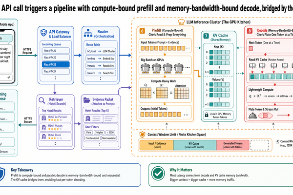
LLM Inference Infrastructure
Next chapter
No adjacent chapter
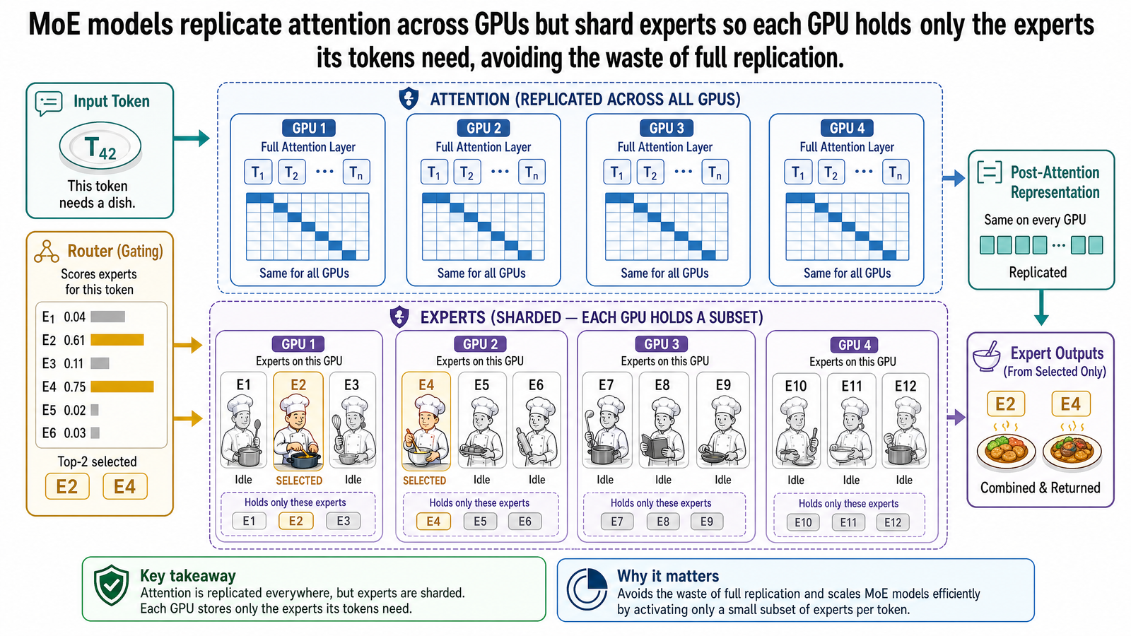
Table of Contents
- What MoE Models Are
- Total Parameters Versus Active Parameters
- Why Simple Replication Does Not Work
- The Replicate-Attention, Shard-Experts Strategy
- Expert Parallelism Explained
- Dynamic Token Routing
- Running Example: Two Queries Through MoE Routing
- The Current MoE Landscape
- Trade-Offs and Failure Modes
- What This Post Is Not
- The Complete Infrastructure Picture
- Source Notes
In Post I-00, we listed five ways that LLM inference differs from conventional model serving. The first four -- variable-length computation, two-phase resource profiles, growing memory requirements, and cache-aware routing -- have each received a full post in this track. The fifth was stated in a single sentence: "Some modern LLMs use a mixture-of-experts architecture, where different parts of the model activate for different inputs. Distributing an MoE model across multiple GPUs requires different sharding strategies than distributing a dense model."
That sentence was deliberately brief because the explanation requires its own foundation. This post provides it. By the end, you will understand why many of the most capable production models -- including DeepSeek-R1, Mixtral, and Llama 4 -- use a fundamentally different internal architecture from the dense models assumed in the previous four posts, and why that architecture demands a different strategy for distributing computation across GPUs.
What MoE Models Are
Every model discussed in this track so far has been a dense model. In a dense model, every parameter participates in every forward pass. When a token passes through a transformer block, it flows through the attention layer and then through a feed-forward network. Every weight in both layers is activated for every token, without exception.
A mixture-of-experts model changes one part of that structure. The attention layer stays the same -- every token still passes through it. But the feed-forward network is replaced by an MoE layer: a collection of N independent feed-forward networks (the experts) and a small routing network (the router, also called the gating network) that decides which experts each token should use.
The router is a learned linear layer that takes a token's representation as input and produces a probability score for each of the N experts. Only the top-k experts -- the ones with the highest scores -- are activated for that token. The rest are skipped entirely. The outputs of the selected experts are combined using the router's scores as weights, and the result is passed to the next layer.
This is sparse activation. The model has N expert feed-forward networks, but each token only uses k of them. If N is 8 and k is 2, each token activates 25% of the expert capacity. If N is 256 and k is 8, each token activates roughly 3%. The remaining experts do no work for that token -- their weights are not read, their computation is not performed, and their outputs are not produced.
The original formulation of this architecture appeared in Shazeer et al.'s "Outrageously Large Neural Networks" (2017), which introduced the sparsely-gated mixture-of-experts layer. Fedus et al.'s Switch Transformers (2022) simplified the routing to top-1 -- a single expert per token -- and demonstrated that MoE could scale to trillion-parameter models while achieving 7x pre-training speedups. These were research milestones. The production impact arrived later.
One clarification matters immediately: experts are not complete models. Each expert is a feed-forward network -- typically two linear transformations with an activation function between them -- within a single transformer block. The experts share the same attention layers, the same embedding layers, and the same output head. An "8-expert MoE model" is not 8 separate models cooperating. It is one model with 8 alternative feed-forward paths per block, selected by the router.
Total Parameters Versus Active Parameters
The sparse activation property creates a distinction that does not exist in dense models: the difference between total parameters and active parameters.
Consider Mixtral 8x7B. The model has 8 experts per MoE layer with top-2 routing. Its total parameter count is 46.7 billion -- that is the sum of all weights across all experts, all attention layers, and all shared components. But because each token activates only 2 of 8 experts, the active parameter count per token is 12.9 billion. The model occupies the memory footprint of a 46.7B model but performs the computation of a 12.9B model for each token.
The ratio is more dramatic at larger scale. DeepSeek-V3 has 256 routed experts plus 1 shared expert per MoE layer, with top-8 routing. Total parameters: 671 billion. Active parameters per token: 37 billion. The model requires memory for 671B parameters, but the compute cost per token is comparable to a 37B dense model -- roughly 5.5% of the total model participates in any given token's forward pass.
This distinction -- total parameters determine memory cost, active parameters determine compute cost -- is the single most important concept in this post. Every serving decision that follows is a consequence of this gap.
Why Simple Replication Does Not Work
In Posts I-01 through I-04, we assumed the model could be replicated across GPUs: copy the full model to each GPU, and each replica independently processes requests. For a dense model, this works. Every parameter on every replica is used for every token. The memory cost is justified by the compute it enables.
For an MoE model, replication is wasteful. If you replicate Mixtral 8x7B across 4 GPUs, each GPU holds all 46.7B parameters. But each token on each GPU only activates 12.9B of them. The remaining 33.8B parameters -- the 6 inactive experts -- sit in GPU memory contributing nothing. Across all 4 GPUs, you have loaded 186.8B parameters total, but only 51.6B are active at any moment. Seventy-two percent of the expert weights are idle on every GPU at every token.
For DeepSeek-V3, the waste is even more stark. Each replica holds 671B parameters but uses only 37B per token. Ninety-four percent of the expert weights sit idle on every GPU. That idle memory could hold KV caches for additional requests, or it could be avoided entirely with a smarter distribution strategy.
The core problem is a mismatch between the memory scaling and the compute scaling. Memory scales with total parameters (all experts must be loaded because the router might select any of them). Compute scales with active parameters (only k experts run per token). Replication pays the full memory cost on every GPU but captures only a fraction of the compute benefit.
The Replicate-Attention, Shard-Experts Strategy
The solution follows directly from the problem. Attention layers and expert layers have different access patterns, so they should be distributed differently.
Attention layers process every token. Regardless of what the router decides, every token in the sequence passes through the same attention computation. The attention weights must be present on every GPU that processes tokens. Replication is the right strategy for attention because every replicated weight is used by every token.
Expert layers are sparsely activated. Each expert processes only the tokens that the router assigns to it. In a model with 8 experts and top-2 routing, each expert handles roughly 25% of tokens on average. There is no reason for every GPU to hold every expert -- most of them will not be needed for the tokens that GPU is processing.
The efficient strategy: replicate the attention layers across all GPUs, and shard the expert layers so each GPU holds a subset of experts. In the simplest case with 8 experts and 8 GPUs, each GPU holds the full attention layers (replicated) plus exactly one expert (sharded). Every parameter on every GPU is used frequently. Nothing sits idle.
As one practitioner described the setup: it is not like having 8 distinct model replicas. It is one large model with routing inside it. The GPUs collectively hold the complete model, but no single GPU holds all of it. Tokens flow through replicated attention on their local GPU, then route to whichever remote GPU holds the expert the router selected.
Expert Parallelism Explained
This distribution strategy has a name: expert parallelism. To understand what makes it distinctive, it helps to contrast it with the two parallelism strategies commonly used for dense models.
Tensor parallelism splits individual layers across GPUs. Each GPU holds a slice of every layer, and all GPUs collaborate on the same computation. After each layer, the GPUs synchronize their partial results via an allreduce operation -- every GPU sends its output to every other GPU, and they all arrive at the same combined result. The communication pattern is static and predictable: the same allreduce happens after every layer, regardless of the input data. This synchronization can contribute up to 30% of end-to-end latency.
Pipeline parallelism splits the model into sequential stages, each assigned to a different GPU. GPU 1 holds layers 1 through 20, GPU 2 holds layers 21 through 40, and so on. Data flows through the pipeline in order: GPU 1 processes its layers and sends the result to GPU 2, which processes the next set of layers and sends the result to GPU 3. The communication pattern is again static and predictable: data always flows in the same direction through the same sequence of GPUs.
Expert parallelism is fundamentally different because its communication pattern is dynamic and data-dependent. Experts are distributed across GPUs, and the router decides at runtime -- based on the actual token representations -- which expert each token needs. Different tokens may route to different GPUs. Different queries may activate entirely different subsets of the expert pool. The system cannot predict in advance which GPUs will communicate with which other GPUs, because that depends on what the router computes for each token.
The communication primitive that enables this is called all-to-all: each GPU can send tokens to any other GPU and receive tokens from any other GPU, based on the routing decisions. This all-to-all pattern occurs twice per MoE layer -- once to dispatch tokens to the GPUs holding their activated experts (the scatter phase), and once to return results to the originating GPUs (the gather phase). According to NVIDIA's measurements, even on well-provisioned clusters, all-to-all communication can contribute 10-30% of end-to-end inference latency. In training workloads across many workers, it can account for 50-60% of total time.
The key tradeoff: tensor and pipeline parallelism have static, predictable communication that can be optimized in advance. Expert parallelism has dynamic, unpredictable communication that depends on the data flowing through the model. This makes expert parallelism harder to optimize but uniquely suited to MoE architectures, where the sparse activation pattern makes static parallelism strategies wasteful.
Dynamic Token Routing
Let us walk through the routing process step by step within a single MoE layer.
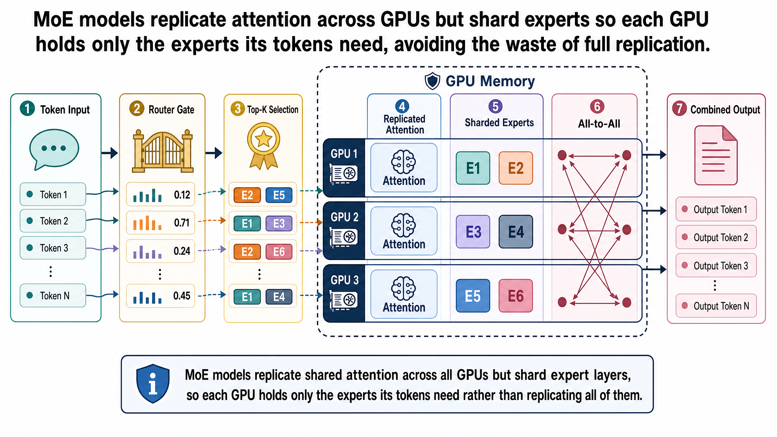
Step 1: Shared attention. All tokens pass through the attention layer on their local GPU. This computation is identical on every GPU -- the attention weights are replicated, so every GPU can process any token's attention independently. At this point, tokens have not yet diverged.
Step 2: Router scoring. The router takes each token's post-attention representation and scores all N experts. For a model with 8 experts, the router produces 8 scores per token. A softmax converts these scores into a probability distribution. The top-k experts are selected.
Step 3: Dispatch (all-to-all scatter). Tokens are sent to the GPUs holding their activated experts. If a token needs expert 5 and expert 5 lives on GPU 5, that token's data is transmitted from whatever GPU processed its attention to GPU 5. This is the first all-to-all communication step -- tokens fan out from their source GPUs to their destination GPUs based on the routing decision.
Step 4: Expert computation. Each GPU processes the tokens that arrived for its local expert. GPU 5 processes all tokens routed to expert 5, regardless of which GPU those tokens came from. This is a standard feed-forward computation -- the same two linear transformations that a dense model would perform, but applied only to the subset of tokens assigned to this expert.
Step 5: Gather (all-to-all gather). Results are returned from the expert GPUs back to the originating GPUs. GPU 5 sends each token's output back to the GPU where that token's attention was computed.
Step 6: Combination. On the originating GPU, the outputs from the top-k experts are combined using the router's probability scores as weights. If a token activated experts 2 and 5 with scores of 0.6 and 0.4, the combined output is 60% from expert 2 and 40% from expert 5. This combined output is passed to the next transformer block.
This entire process repeats at every MoE layer in the model. A model with 60 MoE layers performs 60 rounds of routing, dispatch, expert computation, and gathering -- with two all-to-all communications per layer, that is 120 inter-GPU communication events per forward pass.
Running Example: Two Queries Through MoE Routing
Return to the travel copilot from the main series. Imagine it uses an MoE model with 8 experts per MoE layer, top-2 routing, deployed across 8 GPUs. Each GPU holds the full replicated attention layers plus one expert: GPU 1 holds expert 1, GPU 2 holds expert 2, and so on.
Query A -- hotel availability:
Show me wheelchair-accessible hotels in Kyoto under $200/night with onsen access.
The query's tokens pass through the replicated attention layer. The router scores all 8 experts and selects expert 2 and expert 5 as the top-2 for these tokens. Tokens dispatch via all-to-all communication to GPU 2 (holding expert 2) and GPU 5 (holding expert 5). Each expert processes the tokens routed to it. Results gather back to the originating GPU. The weighted outputs from experts 2 and 5 are combined and passed to the next layer.
Query B -- flight comparison:
Compare direct flights from Tokyo to Osaka on April 15, sorted by departure time.
Same attention computation, same replicated weights, same GPUs. But the router selects different experts: expert 1 and expert 4. Tokens dispatch to GPU 1 and GPU 4. Different GPUs activate for a different query.
The contrast illustrates the core property: the attention path is identical for both queries (every token through every GPU's replicated attention), but the expert path is query-dependent (different GPUs activate based on which experts the router selects). In a replication strategy, all 8 GPUs would hold all 8 experts, and 6 experts would sit idle on every GPU for every query. In the expert parallelism strategy, each GPU holds exactly one expert, and that expert processes tokens from across the entire system.
A note on the expert labels: this example uses shorthand like "structured data" or "travel domain" as pedagogical labels for the experts. In practice, expert specialization is emergent -- it arises from the training process and may or may not align with human-interpretable categories. Research has shown that experts sometimes develop recognizable specializations, but this is an empirical finding, not a design guarantee.
The Current MoE Landscape
MoE is not a research curiosity. As of early 2026, it is the dominant architecture for frontier models.
DeepSeek-V3 (December 2024): 671B total parameters, 37B active per token. 256 routed experts plus 1 shared expert per MoE layer. Top-8 routing. Uses an auxiliary-loss-free strategy for load balancing.
DeepSeek-R1 (January 2025): Same MoE architecture as DeepSeek-V3 (671B total, 37B active), applied to a reasoning-focused model trained with reinforcement learning. Demonstrates that MoE extends beyond standard language modeling to reasoning-intensive workloads.
Mixtral 8x7B and 8x22B (January 2024): 46.7B total, 12.9B active (8x7B). 8 experts per layer, top-2 routing. The first widely adopted open-source MoE model. Matched or exceeded Llama 2 70B on benchmarks while being substantially faster to serve.
Llama 4 Scout (April 2025): 109B total parameters, 17B active. 16 experts per layer, top-1 routing. Meta's first MoE architecture, marking the Llama family's departure from dense models.
Llama 4 Maverick (April 2025): Approximately 400B total parameters, 17B active. 128 experts per layer. The same active parameter count as Scout but with 8 times more experts, offering greater model capacity at the same per-token compute cost.
GPT-4 (March 2023): Often discussed in industry commentary as a possible MoE system, but OpenAI has not officially confirmed its architecture. Treat GPT-4 MoE claims as rumor, not as an architectural fact.
The pattern is clear without relying on unconfirmed models. NVIDIA reports that the top open-source models on inference benchmarks use MoE architectures, and major model builders including Meta, Mistral, and DeepSeek have published MoE systems. The architecture went from a research proposal in 2017 to a mainstream production choice in less than eight years.
The reason is the gap between total and active parameters. MoE lets model builders scale capacity -- the total knowledge and capability encoded in the weights -- without proportionally scaling the compute cost of serving each token. A 671B-parameter model that computes like a 37B model at inference time is a better product economics proposition than a 671B dense model that requires 671B parameters of computation for every token.
Trade-Offs and Failure Modes
MoE is not universally superior to dense architectures. The benefits come with costs that matter in production.
Load imbalance. If the router consistently sends most tokens to the same few experts, those GPUs become bottlenecks while others sit underutilized. A "popular" expert overwhelms one GPU while seven others idle. This manifests as high latency variance and degraded aggregate throughput. Training-time auxiliary losses and inference-time capacity limits help, but load imbalance remains an active engineering challenge.
All-to-all communication overhead. Expert parallelism requires two all-to-all communications per MoE layer. On clusters with limited inter-GPU bandwidth -- particularly when expert parallelism spans across nodes connected by slower network interconnects rather than high-speed intra-node links -- this communication can dominate inference latency, negating the compute savings of sparse activation.
Memory overhead. Despite sparse activation, all experts must be loaded into GPU memory. The router can assign any token to any expert, so no expert can be safely unloaded. The memory requirement scales with total parameters, not active parameters. Expert parallelism distributes this cost across GPUs, but the aggregate memory requirement remains.
Hardware-dependent strategy selection. Expert parallelism is not always the right choice, even for MoE models. AMD's ROCm vLLM MoE Playbook recommends tensor parallelism over expert parallelism on single-node MI300X deployments due to the XGMI bandwidth characteristics of that hardware. The optimal parallelism strategy depends on the number of experts, the number of GPUs, the interconnect topology, and the bandwidth between them. In practice, large deployments often combine expert parallelism with tensor parallelism and pipeline parallelism simultaneously -- a hybrid strategy that is beyond the scope of this post.
What This Post Is Not
This post teaches how MoE models are served. It does not teach how they are trained. Auxiliary load-balancing losses, expert capacity factors, token dropping during training, and MoE fine-tuning techniques are training-time concerns that shape the model's behavior but do not directly determine how the trained model is deployed for inference.
This post also does not teach how to build an MoE inference engine. It teaches what engines like vLLM and SGLang do when they encounter an MoE model and why the default dense-model serving strategies are insufficient. The goal is architectural understanding, not implementation.
Finally, this post does not cover advanced multi-dimensional parallelism -- the practice of combining expert parallelism with tensor parallelism, pipeline parallelism, and data parallelism in a single deployment. Production systems at frontier scale routinely use these combinations. The concepts introduced here -- which components to replicate, which to shard, and why communication patterns differ -- are the foundation for understanding those more complex configurations.
The Complete Infrastructure Picture
This is the final post in the infrastructure track. Across six posts, we have traced the journey from a single API call to the full serving stack that makes production LLM inference possible.
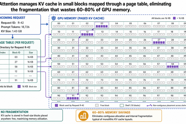
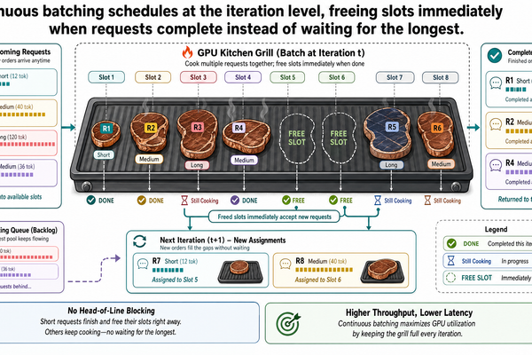
In I-00, we opened the pipeline: attention computes relationships between tokens, the KV cache stores the results, prefill and decode have opposite hardware bottlenecks, and the GPU is a shared resource under contention. In I-01, we solved the batching problem: continuous batching schedules at the iteration level, allowing requests to enter and exit the GPU independently rather than waiting for the slowest request in a static batch. In I-02, we solved the memory problem: paged KV cache management borrows ideas from operating system virtual memory to eliminate the fragmentation that wastes 60-80% of cache capacity. In I-03, we separated the phases: prefill-decode disaggregation runs each phase on hardware matched to its bottleneck, because a compute-bound phase and a memory-bandwidth-bound phase should not compete for the same resources. In I-04, we made routing intelligent: prefix-aware scheduling directs requests to the replica that has already cached their shared prefix, avoiding redundant prefill computation across replicas. And in this post, I-05, we addressed what happens when the model itself is not dense -- when sparse activation means the model's own architecture dictates how it should be distributed across GPUs.
These are the five serving innovations that transformed LLM inference from a research curiosity into production infrastructure: continuous batching, paged memory, phase disaggregation, cache-aware routing, and model-aware sharding. Each solves a different problem. Together, they explain why specialized inference engines exist and why general-purpose serving frameworks are insufficient for LLM workloads.
The application-layer series covers what you build on top of this infrastructure -- compound AI systems, retrieval pipelines, tool use, agents, and evaluation. This track covered what happens beneath it. Together, they give you the complete picture: from the system prompt your application assembles, through the API call, into the GPU pipeline, across the batching and memory and routing decisions, through the model's own internal architecture, and back out as streamed tokens that your user sees as a response.
Source Notes
This post draws on the following primary and practitioner sources:
Shazeer, N., Mirhoseini, A., Maziarz, K., et al. "Outrageously Large Neural Networks: The Sparsely-Gated Mixture-of-Experts Layer." ICLR, 2017. The foundational paper introducing the sparsely-gated MoE layer and top-k expert selection. arxiv.org/abs/1701.06538
Fedus, W., Zoph, B., Shazeer, N. "Switch Transformers: Scaling to Trillion Parameter Models with Simple and Efficient Sparsity." JMLR, 2022. Simplified MoE routing to top-1, demonstrated trillion-parameter scaling and 7x pre-training speedup over T5-XXL. arxiv.org/abs/2101.03961
Jiang, A.Q., Sablayrolles, A., Mensch, A., et al. "Mixtral of Experts." Mistral AI, January 2024. Technical report for Mixtral 8x7B: 46.7B total parameters, 12.9B active, 8 experts per layer, top-2 routing. arxiv.org/abs/2401.04088
DeepSeek-AI. "DeepSeek-V3 Technical Report." December 2024. 671B total parameters, 37B active, 256 routed experts plus 1 shared expert, top-8 routing, auxiliary-loss-free load balancing. arxiv.org/abs/2412.19437
DeepSeek-AI. "DeepSeek-R1: Incentivizing Reasoning Capability in LLMs via Reinforcement Learning." January 2025. Confirms MoE architecture extends to reasoning-focused frontier models. arxiv.org/abs/2501.12948
Meta. "The Llama 4 herd: The beginning of a new era of natively multimodal AI innovation." April 2025. Confirms Llama 4 Scout (109B total, 16 experts, top-1) and Maverick (~400B total, 128 experts). ai.meta.com/blog/llama-4-multimodal-intelligence/
NVIDIA. "Mixture of Experts Powers the Most Intelligent Frontier AI Models." 2025. Industry-level confirmation that top open-source inference benchmark models use MoE. blogs.nvidia.com/blog/mixture-of-experts-frontier-models/
NVIDIA. "Scaling Large MoE Models with Wide Expert Parallelism on NVL72 Rack Scale Systems." Developer Blog. Quantification of all-to-all communication overhead in MoE training and inference. developer.nvidia.com/blog/scaling-large-moe-models-with-wide-expert-parallelism-on-nvl72-rack-scale-systems/
Meta Engineering. "Scaling LLM Inference: Innovations in Tensor Parallelism, Context Parallelism, and Expert Parallelism." October 2025. Production-grade reference for expert parallelism with two-shot all-to-all communication. engineering.fb.com/2025/10/17/ai-research/scaling-llm-inference-innovations-tensor-parallelism-context-parallelism-expert-parallelism/
BentoML. "Data, tensor, pipeline, expert and hybrid parallelism." LLM Inference Handbook. Accessible practitioner comparison of parallelism strategies and their communication patterns. bentoml.com/llm/inference-optimization/data-tensor-pipeline-expert-hybrid-parallelism
AMD. "The vLLM MoE Playbook: A Practical Guide to TP, DP, PP and Expert Parallelism." ROCm Blogs. Hardware-dependent parallelism strategy recommendations for MoE models. rocm.blogs.amd.com/software-tools-optimization/vllm-moe-guide/README.html
Hugging Face. "Mixture of Experts Explained." Accessible reference for MoE gating mechanics and load-balancing concepts. huggingface.co/blog/moe
Huang Tzu Lin
With over five years in autonomous robotics, there's a strong passion for incorporating cutting-edge technologies and innovative approaches. Dedicated to transforming the latest research and insights into practical applications, this journey pushes the limits of possibility.
Related Posts
Stay Updated
Get the latest technical insights delivered to your inbox.